Deep Learning - develop a Long Short Term Memory (LSTM) network for time series analysis using Python

Long Short Term Memory (LSTM) network for time series analysis using Python

 In this document, students can enhance their skills in time series analysis by building a Long Short Term Memory (LSTM) network using Python. LSTM is a specific type of Recurrent Neural Network (RNN) known for its ability to accumulate propagation state throughout the input sequence. This means that the model's output from one timestep becomes the input for the subsequent timestep, allowing the model to make predictions based on both current and prior input, resulting in more reliable prediction outcomes. The persistent accumulation of propagation state is the primary advantage of LSTM models.

 The specific tasks include:

1. define a many-to-many type sequence prediction problem, such as power consumption forecast for next 3 days

2. Design and develop an LSTM neural network with multiple input time steps and multiple output time steps

3. Design an evaluation metric

4. Conduct performance analysis of the LSTM model via training and testing on appropriate data sources

"If you need the complete report and codes, please leave a comment on this blog. Few screenshots, steps, and codes are not included assuming that

 you are able to figure them out. If you are having difficulty getting the output, then please leave a comment and I will help you with that."

Abstract—Pollution is one of the major factors for environmental and climate changes across the world. Also, due to pollutions we are facing many health issues. The pollutions are different types such as, air pollution, water pollution, soil pollution, sound pollution etc. It can be due to the natural calamities like volcano, landslide, wide fire, etc., and pollution can happen because of the human activities. Among all those pollutions, the world is facing air pollution more and it badly effecting the environmental changes and climate changes. There are so many issues we are facing because of  air pollution, so that, in order to predict the pollution and weather changes, this report will analyze five years of weather and level of pollution at each hours and the report prepared by US embassy at Beijing, China.  We used the open dataset Beijing PM2.5 data set from UCI machine learning repository. This assignment uses a Long Short-Term Memory (LSTM) method to predict the weather and level of air pollution in the next hour based on the real dataset. The result gotten from the output of the program indicates that Long Short-Term Memory (LSTM) can effectively predict the weather or level of pollution in the next hour because of its ability to store data and use that stored data, it can be historical or past data to be used for present and future prediction. This assignment is completely based the Long Short-Term Memory (LSTM) network development for time series analysis with the use of python. 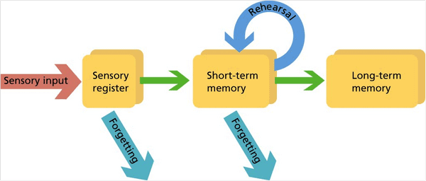Long Short-Term Memory (LSTM) is type of Recurrent neural Network and its main feature is that it can be able to remember its input and also, they can use this input to predict the future outcome. Long Short-Term (LSTM) is a sequence model in which when an input is provided and once the output is produced then that output can be used for the input in the subsequent time step of the model. Long Short-Term Memory (LSTM) makes a model to predict the next timesteps and advanced information gotten from the past timesteps thereby result in more stable prediction result. In this assignment we are going to look at how e can use many -to- many type sequence prediction problem to forecast weather and level pollution for the next hour using the past historical data. Also develop a Long Short-Term memory (LSTM) neural network with many inputs time steps and multiple output time steps, and the evaluation metric will be designed, and performance analysis of the Long Short-Term Memory was done to model the Long Short-Term Memory (LSTM) through training and testing on the dataset I have selected.

                                                              I.    Introduction

       In today’s world predictions have integral part in humans’ life. Every day we except something good or bad will come in our life on the present and previous situations we faced. Also, nowadays, we use machine learning approach to solve most of the future problem by predicting it today itself. The deep learning improved on predictions and machine learning approach used for solving many statistical problems. One of the biggest problems handled by the machine learning approach is weather forecasting and predicting level of pollutions. However, due to the limitations of machine learning the predictions will not be hundred percentage accurate, so that we need to develop another system which can make accurate predictions on weather and level pollutions. With the use of advance level of Deep learning methods, we can develop system which can recognize and predict accurately. Recurrent Neural Network was introduced in which Long Short-Term Memory is a type was adopted because of its ability to store information or data that is past and been able to use it to predict the future.

The main challenge is to get the accurate result, in order to get accurate result and accurate dataset was collected from open source and the data was organized to be able to fit into the network to learn the input sequence effectively. At the end, we will compare the actual and predicted data series that was obtained and then data was evaluated, and prediction was made by the use of python program to run the result in which evaluation metric was used. Finally, the result accurately shows that Long Short-Term Memory as greatly improved the prediction of weather and level of pollution.

More about Long Short-Term Memory Network

Hochreiter and Schmidhur invented the Long Short-Term Memory (LSTM) network in 1997 and it is used for problems in multiple application domains. The ability to recognize feature of LSTM gained more prominence in the area of speech recognition, also in 2009 Long Short-Term Memory network became the first Recurrent Neural Network to win handwriting recognition. The Long Short-Term network is a type of Recurrent Neural Network that has the ability to extend the memory, is a building block for most layers of recurrent neural network. It has the ability assign data to either let new information to get in or forget information or improved on it to produce a good output. Long Short-Term Memory helps recurrent neural networks to always remember the input for a long period of time, because it stores its information in a memory, like the memory of a computer Long Short-Term Memory can write, read, and can also delete information stored in its memory. Long Short-Term Memory (LSTM) allows a model to predict the next timestep with regards to the input for the current timesteps and advanced information gotten from the past timesteps thereby result in more stable to look at how we can use many-to-many type sequence prediction problem to forecast weather and level of pollution for next hours using the past input to derive its future. Also develop Long Short-Term Memory neural network with many input timesteps and multiple output time steps, and the evaluation metric will be designed, and performance analysis of the Long Short-Term Memory was done to model the Long Short-Term through training and testing on the chosen sets.

The major goal and advantage of a Long Short-Term Memory which is a type of a recurrent neural network is that it enables the model to make a prediction on the input for the recent timesteps and the knowledge derived in the past timesteps resulting in the accurate prediction of the new result. Recurrent neural network which Long Short-term Memory is a type of can be classified as a neural network that can be very useful in the modelling of sequential data in prediction of future result. It has the ability to retain past input and use it for the present and then used it to predict the future, this makes it to stand out among other algorithms.

Long Short-Term Memory function with working knowledge for feed forward neural networks and sequential date. Long Short-Term cannot function if the data that is given are not sequential or in the order i.e., a data that is related follow each other. Long Short-Term can be used to predict wat will happen in the future or if there is a painful situation and how it will affect it. Time series data is the most popular type of sequential data.

A.   Proposed Model

Predicting the weather conditions and level of pollution in the next hours is one of the important tasks and one of the predictions that everyone waiting for. Due to many unpredictable circumstances sometimes, the predictions may not be accurate, or it will be completely a wrong prediction. The machine learning techniques has limitations to overcome the unpredictable situations, so that in this assignment we use Long Short-Term Memory networks, which is a specific kind of recurrent neural network. Long Short-Term Memory network has the ability to correlate the previous information and present prediction results. In weather forecasting and level of pollution prediction LSTM will be more effective to provide more accurate prediction results.

In this assignment, I have used a dataset from UCI machine learning repository, which has the past 5 years hourly data of weather and level of pollution in Beijing, China. I will briefly explain what the things are included in the datatset. It comes with, date and time, which means year, month, day and hour, also the pollution concentration mentioned and pm2.5 and the other weather information like dew, temperature, pressure, wind speed etc. With this dataset, we will get the weather condition and pollution for prior hours so that we can use this information to predict the pollution at the next hour.

In order to use that dataset first we complete the data preparation. I will include the first 5 rows of the dataset we downloaded from UCI machine learning repository.

First, we have to change the date and time information into a single date and time so that while using the Pandas we can use date-time as an index. We can see that pm2.5 column shows NaN values for the past 24 hours, so that we need to change that to 0 values which means NA values will be replaced with 0. The date-time information will be sent to the Pandas DataFrame index, since we are using date-time as index we will drop the “No” column.

Now we have to load the dataset, I have loaded the dataset by parsing date-time as Pandas DataFrame index and dropping” No” column and replacing NA with 0. Also, the modified dataset remained and saved as “pollution.csv”

from math import sqrt
from numpy import concatenate
from matplotlib import pyplot
from pandas import read_csv
from pandas import DataFrame
from pandas import concat
from sklearn.preprocessing import MinMaxScaler
from sklearn.preprocessing import LabelEncoder
from sklearn.metrics import mean_squared_error
from keras.models import Sequential
from keras.layers import Dense
from keras.layers import LSTM
from datetime import datetime
# load data
def parse(x):
 return datetime.strptime(x, '%Y %m %d %H')
dataset = read_csv('PRSA_data_2010.1.1-2014.12.31.csv',  parse_dates = [['year', 'month', 'day', 'hour']], index_col=0, date_parser=parse)
dataset.drop('No', axis=1, inplace=True)
# manually specify column names
dataset.columns = ['pollution', 'dew', 'temp', 'press', 'wnd_dir', 'wnd_spd', 'snow', 'rain']
dataset.index.name = 'date'
# mark all NA values with 0
dataset['pollution'].fillna(0, inplace=True)
# drop the first 24 hours
dataset = dataset[24:]
# summarize first 5 rows
print(dataset.head(5))
# save to file
dataset.to_csv('pollution.csv')

Now we have saved the “pollution.csv” new dataset. Let me plot the 5 years of data for each weather variable with 7 subplots.

The code is,

#sub plots
from matplotlib import pyplot
values = dataset.values
# specify columns to plot
groups = [0, 1, 2, 3, 5, 6, 7]
i = 1
# plot each column
pyplot.figure()
for group in groups:
 pyplot.subplot(len(groups), 1, i)
 pyplot.plot(values[:, group])
 pyplot.title(dataset.columns[group], y=0.5, loc='right')
 i += 1
pyplot.show()

And the 7 subplots without wind speed direction, we are excluding since it is a categorical variable.

Which means, we have prepared our data for developing Long Short-Term Memory network model.

                                     II.    Design and Develop of an LSTM

We are all set to develop the Long Short-Term Memory network model to predict the next hour pollution.

A)    Define many-to-many sequence prediction problem

Many-to-many is one of the Recurrent Neural

Network models in which it will generate output whenever each input is read. Our dataset we can convert in to supervised learning problem with the help of series_to_supervised() function. Also, the wind direction is a categorical variable and we can represent it as binary variable. By using the many-to-many sequence prediction lets predict the pollution level at the current hour.

# input sequence (t-n, ... t-1)
for i in range(n_in, 0, -1):
    cols.append(df.shift(i))
    names += [('var%d(t-%d)' % (j + 1, i)) for j in range(n_vars)]
# forecast sequence (t, t+1, ... t+n)
for i in range(0, n_out):
    cols.append(df.shift(-i))
    if i == 0:
        names += [('var%d(t)' % (j + 1)) for j in range(n_vars)]
    else:
        names += [('var%d(t+%d)' % (j + 1, i)) for j in range(n_vars)]

This code will provide the transformed dataset below,

The transform dataset comes with 5 rows and 9 columns with 8 input series (input variables) and 1 output series(variable) which will be the pollution level at current hour.

B)    Design and Develop an LSTM neural network

     We have already discussed about the providing multiple input timesteps and output timesteps. The first steps for developing Long Short-Term Memory network is to prepare the dataset, in this assignment we will prepare pollution dataset. We need to transform the dataset to a supervised learning problem and also need to normalize input variables. By making the supervised learning problem we will predict the pollution at current hour by using the pollution measurement and weather conditions at the previous timestep. With this formulation by using the last 24 hours weather condition and pollution we can predict the next hour pollution and also the weather condition of next hour. As, we discussed earlier, we need to represent the categorical wind direction to binary. Once all the features are normalized then the dataset will convert into a supervised learning problem.

We can define the LSTM model once we split the training and testing sets. We will explain in detail about it in the Section II D.  It is always better to explain the splitting dataset in to training and testing and defining Long Short-Term Memory network model together.  In brief, I would like to say, I am planning to define the LSTM model like first hidden layer with 50 neurons and outer layer with 1 neuron for predicting pollution. Which means the shape of input will be 1 time step with 8 features.

# convert series to supervised learning
def series_to_supervised(data, n_in=1, n_out=1, dropnan=True):
    n_vars = 1 if type(data) is list else data.shape[1]
    df = DataFrame(data)
    cols, names = list(), list()
    # input sequence (t-n, ... t-1)
    for i in range(n_in, 0, -1):
        cols.append(df.shift(i))
        names += [('var%d(t-%d)' % (j + 1, i)) for j in range(n_vars)]
    # forecast sequence (t, t+1, ... t+n)
    for i in range(0, n_out):
        cols.append(df.shift(-i))
        if i == 0:
            names += [('var%d(t)' % (j + 1)) for j in range(n_vars)]
        else:
            names += [('var%d(t+%d)' % (j + 1, i)) for j in range(n_vars)]
    # put it all together
    agg = concat(cols, axis=1)
    agg.columns = names
    # drop rows with NaN values
    if dropnan:
        agg.dropna(inplace=True)
    return agg


# load dataset
dataset = read_csv('pollution.csv', header=0, index_col=0)
values = dataset.values
# integer encode direction
encoder = LabelEncoder()
values[:, 4] = encoder.fit_transform(values[:, 4])
# ensure all data is float
values = values.astype('float32')
# normalize features
scaler = MinMaxScaler(feature_range=(0, 1))
scaled = scaler.fit_transform(values)
# frame as supervised learning
reframed = series_to_supervised(scaled, 1, 1)
# drop columns we don't want to predict
reframed.drop(reframed.columns[[9, 10, 11, 12, 13, 14, 15]], axis=1, inplace=True)
print(reframed.head())

C)   Design an evaluation metric

Once we define and fit the model then we can start forecasting for the test dataset we have made. First, in order to forecast we need to combine the forecast with the test dataset and the reverse data scaling (invert the scaling). Also, need to invert the expected pollution numbers in the test dataset.  After that we are able to calculate the error score for the model we developed, for that we need to use the forecasts and actual values in the original scale. Once we calculate the error score then we can find the Root Mean Squared Error (RMSE). The evaluation performed by using the Mean Absolute Error (MAE) loss function performance metric function.

 make a prediction
yhat = model.predict(test_X)
test_X = test_X.reshape((test_X.shape[0], test_X.shape[2]))
# invert scaling for forecast
inv_yhat = concatenate((yhat, test_X[:, 1:]), axis=1)
inv_yhat = scaler.inverse_transform(inv_yhat)
inv_yhat = inv_yhat[:, 0]
# invert scaling for actual
test_y = test_y.reshape((len(test_y), 1))
inv_y = concatenate((test_y, test_X[:, 1:]), axis=1)
inv_y = scaler.inverse_transform(inv_y)
inv_y = inv_y[:, 0]
# calculate RMSE
rmse = sqrt(mean_squared_error(inv_y, inv_yhat))
print('Test RMSE: %.3f' % rmse)

We will explain more about in the next section, which is for training and testing,

D)   Performance analysis of LSTM model via training and testing.

  Now I will discuss in detail about how to design fit model and how to split the dataset in to test and train sets. I have split the dataset in to test and train and then split the train and test sets in to input and output variables. In order to save time and fast processing we will only use first year of data for training and the left over 4 years of data will be used for evaluation purpose. The inputs will be reshaped with the expected LSTMs 3D format, namely [samples, timesteps, features]

# split into train and test sets
values = reframed.values
n_train_hours = 365 * 24
train = values[:n_train_hours, :]
test = values[n_train_hours:, :]
# split into input and outputs
train_X, train_y = train[:, :-1], train[:, -1]
test_X, test_y = test[:, :-1], test[:, -1]
# reshape input to be 3D [samples, timesteps, features]
train_X = train_X.reshape((train_X.shape[0], 1, train_X.shape[1]))
test_X = test_X.reshape((test_X.shape[0], 1, test_X.shape[1]))
print(train_X.shape, train_y.shape, test_X.shape, test_y.shape)

The above code will provide the train and sets input and output shapes which is about 8760 hours of training data and about 35039 hours for testing.

Since we got the training and testing set, we can now define the LSTM model. As I informed earlier, the first hidden layer of LSTM comes with 50 neurons and the output layer with 1 neuron for predicting pollution. The shape of the input will be 1 time step with 8 features. Also, will use MAE (Mean Absolute Error).

There will be 50 training epochs and the batch size will be 72. By using the validation_data argument in the fit() function , finally, we will trach both training and test loss during training.

# design network
model = Sequential()
model.add(LSTM(50, input_shape=(train_X.shape[1], train_X.shape[2])))
model.add(Dense(1))
model.compile(loss='mae', optimizer='adam')
# fit network
history = model.fit(train_X, train_y, epochs=50, batch_size=72, validation_data=(test_X, test_y), verbose=2,
                    shuffle=False)
# plot history
pyplot.plot(history.history['loss'], label='train')
pyplot.plot(history.history['val_loss'], label='test')
pyplot.legend()
pyplot.show()

Also, it will create a plot which will shows the loss of training and testing during training.   I will add the screenshot of plot and epochs.

i.               Line plot of train and test loss

     By looking at the plot, we can understand that test loss drops below training loss which means the model I created may be overfitting the training data. We can also check the train and test loss at the end of each epoch, I will add the screenshot for each epoch.

Once it complete 50 epochs and plot is printed then finally it will print the RMSE of the model on the test dataset.

The RMSE achieved by the model is 26.605 which is lower than RMSE found with a persistence model.

Conclusion

In this assignment we discussed about LSTM, many-to-many model, defining, developing and evaluating LSTM and finally training the data to predict the pollution. Modelling of weather forecast, and prediction of pollution is a challenging task since it will depend other factors as well like natural calamities. In this context, this assignment proposes a powerful Long Short-Term Memory model-based weather forecasting and pollution prediction model which is validated by using the hourly based data collected dataset. We also used MAE (Mean Absolute Error) loss function to evaluate the metrics. We aim to collect more data to test and verify the predicted variable of our proposed model as the further research work.

"If you need the complete report and codes, please leave a comment on this blog. Few screenshots, steps, and codes are not included

 assuming that you are able to figure them out. If you are having difficulty getting the output, then please leave a comment and I will help

 you with that."

References

 

1.     R. S. Sutton and A. G. Barto, Reinforcement Learning: An Introduction, Cambridge, MA:MIT Press, 1998.  

2.     Jason Brownlee PhD , Multivariate Time Series Forecasting with LSTMs in Keras https://machinelearningmastery.com/multivariate-time-series-forecasting-lstms-keras/

3.     M. A. Wiering, "Explorations in efficient reinforcement learning", February 1999. J. Clerk Maxwell, A Treatise on Electricity and Magnetism, 3rd ed., vol. 2. Oxford: Clarendon, 1892, pp.68–73.

4.     Dargan, S., Kumar, M., Ayyagari, M.R. and Kumar, G., 2020. A survey of deep learning and its applications: a new paradigm to machine learning. Archives of Computational Methods in Engineering, 27(4), pp.1071-1092.

5.     Https://machinelearningknowledge.ai/basic-understanding-of-environment-and-its-types-in-reinforcement-learning/#1_Deterministic_vs_Stochastic_Environment

6.     Melo, Francisco S. "Convergence of Q-learning: a simple proof"